

| Victor Malyshkin | Galina Dudnikiva | ||||
| Marina Kraeva | Vitaly Vshivkov | ||||
| Supercomputer Software Department, Computing Centre RAS |
Institute of Computing Technologies RAS |
||||
| Novosibirsk, RUSSIA | Novosibirsk, RUSSIA | ||||
|
|
This work is partially supported by the grants ITDC-203 and RFBR 96-01-01557
V.Malyshkin. Functionality in ASSY System and Language of Functional Programming. Proc. "The First Aizu International Symposium on Parallel Algorithms/Architecture Synthesis", 1995, Aizu-Wakamatsu, Fukushima, Japan. IEEE Comp. Soc. Press, Los Alamitos, California. P. 92-97.
V.Vshivkov, M.Kraeva, V.Malyshkin. Parallel Implementations of PIC Method. "Programmirovanie", 1996
Parallel programming, Assembly technology, Particle-in-cell method
The subject of our research is assembly method of parallel programs construction for supporting the numerical big size problems solution on MIMD computers. In particularly we are developing the parallel programming language and system including automatic parallel programs synthesis subsystem. As example of big size problem we consider plasma physics problems that are solved by Particle-in-cell (PIC) method. The control structure of parallel program that implement this problem solving algorithm essentially depends on input data structure and volume. Thus it's necessary to construct special parallel program for each new input data.
PIC is now one of the most popular method in different natural phenomena investigations. The success of PIC is due to the ability of this method to mimic true plasma behaviour. With the PIC model a plasma is represented in the same way as a real plasma appears: as a lot of particles immersed in and evolving with an electromagnetic field. This popularity of the method demands the development of successful tool. We will discuss here the general scheme of computation only and the problem of its parallelization. Consider PIC method in its application to solution of the collisionless interaction of plasma flows problem. The model for this problem description is equations system that consists of kinetic Vlasov's equations for ions and electrons (in 7-dimensional space: 3 co-ordinates of physical space, time and 3 co-ordinates of particles velocities) and Maxwell's equations:
Current density and charge density are determined from distribution functions:
![]()
Vlasov's equations characteristics describe the tracks of particles moving. Then more particles are involved to model plasma behaviour then more precise result of modelling is computed.
Vlasov's equations are discretized, discrete moving of the particles is described by the system of difference equations. From the viewpoint of problem solution PIC provides the reduction of the 7- dimensional problem to the 3-dimensional problem of the particles tracks computing inside the space of modelling.
So, in PIC simulations plasma is represented as a large number of "superparticles" each of which models the action of a large number of physical particles. The tracks of these "superparticles" (further we will drop the "super" prefix) are characteristics of Vlasov's equations. The particle is represented by its co- ordinates, its mass m and the values of its own electrical and magnetic fields.
The real physical space is represented as 3-D box, model of physical space (space of modelling). The whole modelling space is devided by rectangular grid into cells upon which the electric and magnetic fields, current density and charge density are discretized.
On the other hand it may be said space of modelling is assembled out of small boxes (cells), fig. 2.
Each cell contains the description of electromagnetic forces (field) effecting inside the cell: electrical E and magnetic H (magnetised background). The values of electrical and magnetic forces in any point inside the cell are calculated by interpolation. The more number of cells the more precision of electrical and magnetic fields representation. These forces effect on the particles located inside the cell.
Each particle has its own electrical and magnetic fields, all these fields influent each other. By the action of these forces the particles are moving inside the space, their own electromagnetic fields change the fields of magnetised background. The new co-ordinates of particles are step wise recalculated from difference equations.
The dynamics of the system is followed by integrating the motion equation of each of the particles in a series of discrete time steps (fig.3)

Schematically the modelling is doing as follows. New co-ordinates of particles inside all the cells are calculated from the function G of type:
P_coordinatesi+1 (ti+1 ) = G (P_coordinatesi , Ei, Bi, ti). ti+1 = ti+dt , Ei = Ei (ti), Bi = Bi (ti)
From the physical considerations the time step and the size of cells are choosen in such a way that a particle can't fly during one time step the distance more long then the size of one cell. Thus, during one time step of modelling a particle is able to fly into neighbour cell only, not more far. In such a way, only the values of electrical and magnetic fields inside the cell and its adjacent cells are involved in computations. Calculations of new (i+1)-th co-ordinates of the particles constitute the odd steps of modelling.
After all the particles were moved to new co- ordinates the values of electrical E and magnetic H forces inside the space of modelling should be recalculated because their values are changed under influence of the electrical and magnetic fields of the particles in their new co-ordinates.
(Ei+1, Bi+1)=G1 (P_coordinatesi+1, Ei, Bi, ti).
These calculations constitute the even steps of modelling. Odd and even steps are loopwise repeated calculating the tracks of the particles. Modelling is terminated from physical reasons.
On MIMD distributed memory computers the performance characteristics of a PIC code depends crucially on how the grid and particles are distributed among the processors. The amount of computations in the scatter, gather and push phases of the PIC algorithm is proportional to the number of particles. The computational cost of the field solve phase is proportional to the number of grid points. Generally this cost much less than for other three phases. The push phase is easy to parallelize (fig. 3). However large amount of grid data needs to be exchanged between processors and load imbalance arises when scatter and gather phases are parallelized.
A parallel PIC code depends on following factors too:
There are a great number of parallel implementations of various problems that were solved by PIC method on specific architectures multicomputers. We have implemented this method in its application to solving the collisionless interaction of plasma flows problem on some parallel computer systems (multiprocessor computer ES-1068.17, multitransputer system that consists of 5 transputers T800-20). And gain methods will be used in subsystem for automatic synthesis of parallel programs realising PIC method. On the whole, development of ASSY (ASsembly SYstems) language and system is based first on the analysis of results of large-size problems solving including their parallelization, design of parallel algorithms, data transferring and communications, programming and debugging.
Contrary to widespread parallelization methods in which a problem, defined as a whole, is divided into the suitable fragments to be executed on the different processor elements, the assembly technology supports explicit assembling of a whole program out of ready made fragments of computations. These fragments are the "bricks" to build the whole program. An algorithm of problem assembling defines the "seams" of a whole computation, the way of the fragments connection. This algorithm is kept by ASSY and used later for program parallelization - the "seams" give to compiler an information for automatic dividing of entire computation along the "seams" in suitable fragments (as data as program code). Thus user describes the problem by using friendly interactive system and nonparallel program language for determination computations in minimal object.
Let us consider assembly technology by the example of description of particle-in-cell method.
Definition of particle, of particle array
particle:array[2](coordinates x,y,z:real; u,v,w,q:real;);
Definition of cell
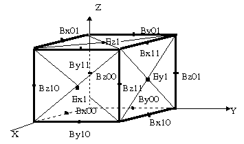
| cell:( | i in N[0,K+1]; |
| j in N[0,K+1]; | |
| k in N[0,M+1]; | |
| Bx00,...,Uz1:array[3]double, Ex0,...,Pz1:array[2]double; | |
| cpart:array of particle); |
Definition of minimal fragment of computations
| box_3x3x3:( | ci,cj,ck:int; cell1=cell: {cell.i==ci,cell.j==cj,cell.k==ck}; ... cell27=cell: {cell.i==ci+1,cell.j==cj+1,cell.k==ck-1,); |
Variables identification
cell26.Bz11 ident cell27.Bz10;
...

Description of operations
...
forall particle in cell1.cpart
| {oper new_param ( | in | particle[0].x,...,particle[0].q,tau,h1,h2,h3,cell1.Bx00[1],... |
| out | particle[1].x,...,particle[1].w,cell1.Px0[0],..., cell5.Uz1[0]) |
};
...);
Assembling of modelling space out of fragments (with covering)
| MS:array[]( | forall ci in N[1,K] forall cj in N[1,L] forall ck in N[1,M] { MS:U(box_3x3x3: {box_3x3x3.ci==ci, box_3x3x3.cj==cj,box_3x3x3.ck==ck}); }; |
The identification of covered cells
forall ci in N[1,K-1]
forall cj in N[1,L-1]
forall ck in N[1,M-1]
{ box_3x3x3.cell1: {box_3x3x3.ci==ci, box_3x3x3.cj==cj, box_3x3x3.ck==ck} ident box_3x3x3.cell8: {box_3x3x3.ci==ci+1, box_3x3x3.cj==cj, box_3x3x3.ck==ck};
...
}; );
Assembly programming technology is destined for numerical solving of various big size problems. Thus we are interesting in studying and solving such complicated applied problems that can't be solved consistently with good success.
This page last updated on April 21, 1997 by Marina Kraeva.